A closer look at “Elaborating and Testing Erotic Target Identity Inversion Theory”

TL;DR: In July, Michael Bailey, Kevin Hsu and Henry Jang published the paper Elaborating and Testing Erotic Target Identity Inversion Theory in Three Paraphilic Samples, claiming to find a correlation 0.95; 1.00; and 1.01 between respectively apotemnophilia and BIID (among acrotomophiles); autozoophilia and cross-species identity (among zoophiles); and autolipophilia and yearning to be fat (among lipophiles). I immediately requested to get the data, and eventually in September, Michael Bailey sent me the data. I replicate their original results using their original methods. Then, I try to correct the methods to be somewhat more precise, and again I replicate their results, finding correlations of 0.95, 1.00 and 1.00 between the interests.

Background

Michael Bailey is the main academic proponent of erotic target identity inversion theory, which is probably most easily understood with an example. Consider the following three phenomena:

1. Male gynephilia, i.e. men’s tendency to be sexually attracted to women.
2. Male autogynephilia, i.e. some male’s tendency to be sexually attracted to being women.
3. Male-to-female transsexuality, i.e. some natal males’ tendency to take female hormones and adopt feminine appearance and social categorization.

These are somewhat related to each other, e.g. gynephilia and autogynephilia tend to cooccur, and autogynephilia and cross-gender identity tend to cooccur. ETII theory asserts that this is due to a causal chain, gynephilia -> autogynephilia -> transsexuality ¹, and that similar phenomena can occur based on a wide variety of sexual interests.

Michael Bailey believes that scientifically demonstrating this pattern of correlations for other targets of attraction than women is a key step in establishing ETIIs as a general phenomenon. Therefore he investigated men who are attracted to amputees, animals and fat people, to see if it generalizes.

In order to recruit people who were attracted to amputees, the researchers got data from many communities devoted to sexual attraction to amputees or to the desire to be an amputee. In order to recruit people who were attracted to animals, they recruited participants from various communities dedicated to zoophilia (and maybe also a few forums dedicated to furries?). In order to recruit people who were attracted to fat people, they recruited from various communities dedicated to that.

In terms of raw correlation between autosexual attraction and self-identity, the researchers found correlations of 0.78, 0.75, and 0.82. However, they felt that this was an underestimate due to measurement error, so they estimated that if it was not for measurement error, the correlations would have really been 0.95, 1.00, and 1.01.

What does this look like?

There is a kind of plot I’ve started to enjoy making:

Basically, I create a variable representing overall apotemnophilia/BIID by combining the scores from the various questions listed in the bottom of the plot. The units of this composite variable are arbitrary, but I have a histogram of it at the top of the diagram. The rows below the histogram show the median response to each question for a given level of the composite variable.

I find this sort of diagram useful because it gives a way to generate a concrete image for what a given level of the composite variable corresponds to; simply trace down vertically from some score and read off what the median response for that score is. So for instance someone who has an overall score of 2.5 would consider it very erotically important to imagine being an amputee in sexual fantasy, would have considered having a limb amputated, and so on.

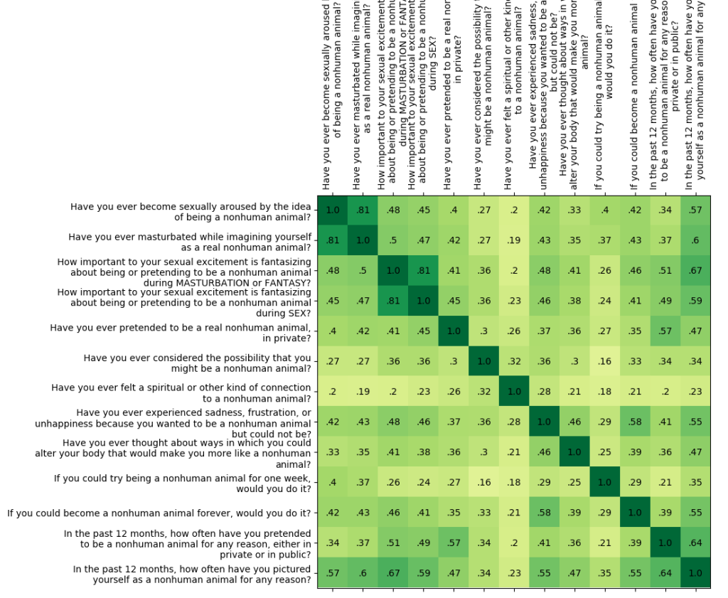
Here is a similar diagram for zoophiles:

And lipophiles:

Anyway, these diagrams are just a bonus visualization, they are not my main topic of investigation, which instead is:

Is the paper’s method valid?

Disclaimer: I have only investigated the validity of their approach from a single angle, so I don’t know whether there are any problems from any other angles.

The initial thing I noticed with their results was that their correlations were really high. Correlations in the 0.7-1.0 range are reasonably common in psychometrics (though my prior investigations in this area had led me to expect correlations more in the 0.4-0.8 range), but it is mathematically impossible for a correlation to exceed 1, so since they got a result of 1.01, obviously their method must be broken somewhere.

The most obvious place to look is in their “correcting for attenuation”, which is basically a fancy statistics term for deciding that the correlation observed in the scores computed from the raw data is an underestimate due to measurement error, and bumping up the correlation relative to what you actually see in order to compensate for that.

This might sound somewhat fishy, but any research is going to be dependent on methods like that. The more interesting question to me is what assumptions it makes, and whether those assumptions apply in this case. In order to justify their use of the method, Bailey et al cite “Encyclopedia of Research Design”, which states correcting a correlation between two tests X and Y for attenuation has two assumptions:

1. The test scores consist of a mixture of “true score” (signal) and “measurement error” (noise).
2. The noise is independent of everything else.

If this seems impossibly abstract to you, then that’s good, because the list here entirely neglects what “measurement error” means or how one can reason about it. But that is important for understanding the method, so let’s dig in.

Internal reliability and Cronbach’s alpha

There are many different notions of “true score” vs “measurement error”. The one used by the researchers in this paper is called “internal reliability”, and it relies on the fact that the test consists of multiple different items.

As an example, the measure of apotemnophilia contains multiple questions, two of which are “Have you ever masturbated while imagining yourself as an amputee?” and “How important to your sexual excitement is fantasizing about being or pretending to be an amputee during SEX?”. In the data, these questions are not independent, but instead have a correlation of 0.56, which we assume is due to the fact that both reflect a sexual attraction to being an amputee. However, if both of the items were perfect indicators of sexual attraction to being an amputee, then they would also have been perfectly correlated with each other, so the fact that the correlation is 0.56 rather than 1.0 makes us infer that there must be some measurement error too.

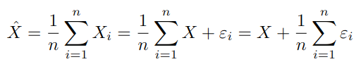
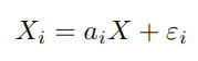
Given this sort of situation, one of the oldest ways of quantifying measurement error can be used. It is called Cronbach’s alpha, and it works as follows: Suppose the test consists of n items, X₁, X₂, …, X_n. Let’s say that each item X_i is the sum of some true score X (e.g. the “true apotemnophilia level”) and some independent measurement error ε_i:

We are then interested in the properties of X̂, which we define to be the estimate of X obtained through averaging all of the X_i, which we can infer to consist of X plus some measurement error:

(The big Σ character is a greek S, and it stands for “sum”, because it represents summing all of the following things together. That is, by definition, ΣX_i = X₁ + X₂ + … + X_n. Since an average is defined by adding a bunch of numbers together and then dividing by the amount of numbers you have, this means the average of X_i can be written as 1/n ΣX_i, as above.)

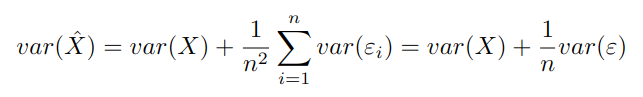
A useful tool for talking about this subject is the statistic known as variance. It is the square of the standard deviation, and while it is hard to intuitively get a feel for, it has the important property that the variance of the sum of some independent variables is the sum of their variances². We assume that the measurement error is independent of everything else (we’ll return to this assumption later), and this lets us express the variance of X̂:

(We end up with the 1/n² factor rather than a 1/n because the original 1/n reduces the standard deviation by a factor of n, and since the variance is the square of the standard deviation, it thereby reduces the variance by a factor of n-squared.)

For further simplicity, we assume that var(ε_i) = var(ε_j); we will return to that assumption later, but it allows us to simplify:

If we now go back to our X_i = X + ε_i equation, compute the variance, scale it down by n, and subtract it from the above, we get:

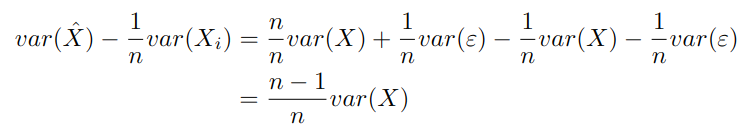
And finally if we rearrange:

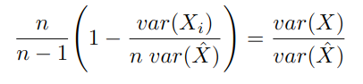
Now, why is the above equation important? Well, the right-hand-side, var(X)/var(X̂) is the ratio of true variance to total variance in the scores, so in a sense it represents the quality of our measurement. On the other hand, the left-hand-side is an expression which solely involves observable quantities in the data, and can therefore be computed directly given the dataset. So if you are willing to grant the assumptions made in the derivation above, this equation allows you to compute the quality of your measure from the statistics of your data.

Correcting for attenuation

OK, so there’s a bunch of times where Bailey et al want to correlate two variables X and Y, e.g. apotemnophilia (X) and body integrity identity disorder (Y). They create a bunch of questions to assess X and Y, e.g. for apotemnophilia:

• Have you ever become sexually aroused while picturing yourself as an amputee?
• Have you ever masturbated while imagining yourself as an amputee?
• How important to your sexual excitement is fantasizing about being or pretending to be an amputee during MASTURBATION or FANTASY?
• How important to your sexual excitement is fantasizing about being or pretending to be an amputee during SEX?

And e.g. for body integrity identity disorder:

• Have you ever pretended to be an amputee?
• Have you ever felt that you were meant to be an amputee?
• Have you ever wished you could become an amputee?
• Would you feel more complete and satisfied if you were an amputee?
• Have you ever felt sad, frustrated, or unhappy because you are not an amputee?
• Have you ever considered trying to become an amputee?
• In the past 12 months, how often have you pretended to be an amputee for any reason, either in private or in public?
• In the past 12 months, how often have you pictured yourself as an amputee for any reason?

Now let’s say we create scores X̂ and Ŷ by averaging the two sets of questions above. One obvious proxy for the correlation between X and Y would be the correlation between X̂ and Ŷ, which in this case I can compute to be 0.76. However, if I compute the Cronbach’s alpha for X̂ and Ŷ, I get α_X̂=0.89 and α_Ŷ=0.92. Since the alpha is less than 1, we can infer that we have measurement error, which means that 0.76 is an underestimate of the true relationship between X and Y. What can we do about that?

The solution is to divide the correlation by √(α_X̂α_Ŷ). I wish I had a quick proof of this that doesn’t rely on elaborate covariance algebra, but unfortunately I don’t. A quick heuristic argument is that a Pearson correlation is standardized by the standard deviation of the variables, and since α_X̂=var(X)/var(X̂), √α_X̂=std(X)/std(X̂), so by dividing by α, we switch out the standardization by the standard deviation of X̂ and Ŷ with a standardization by the standard deviation of X and Y, thereby removing measurement error.

Regardless of the reasoning, this gives us a corrected correlation of 0.76/√(0.89*0.92) = 0.84.

Parceling and correlated measurement error

The attentive among you may have noticed that this correlation of 0.84 is much lower than the correlation of 0.95 that Bailey et al reported between apotemnophilia and body integrity identity disorder. This is because of an additional step they did:

Erotic Target Identity Inversion Theory specifes that a subset of males with every external sexual attraction develops an internalized sexual attraction, experiencing sexual arousal by the fantasy of being an instance of their external erotic target (Hypothesis 1). Table 2 includes descriptive statistics for the two brief subscales used to measure the existence (i.e., presence or absence) and sexual importance of the three respective internalized sexual attractions: apotemnophilia (sexual arousal by the fantasy of being an amputee), autozoophilia (sexual arousal by the fantasy of being an animal), and autolipophilia (sexual arousal by the fantasy of being an obese person). The correlations between the two subscales were 0.63, 0.53, and 0.61, respectively, for the three samples (ps<.001). Both subscales were standardized and averaged for each sample to produce a composite measure of internalized sexual attraction for subsequent analysis. Table 2 also includes Cronbach’s alpha for each sample’s composite measure.

(emphasis added)

Erotic Target Identity Inversion Theory specifes that men with internalized sexual attractions will sometimes develop erotic target identity inversions, refecting a wish or desire to become their external sexual attractions (Hypothesis 2). Table 3 includes descriptive statistics for the two subscales intended to measure erotic target identity inversions in the three samples, which would correspond with apotemnophilia, autozoophilia, and autolipophilia. The first subscale assessed whether participants had ever experienced feelings or behaviors indicating erotic target identity inversions, and the second subscale assessed participants’ frequency of self-imagining or imitating their specifc atypical erotic target. The correlations between the two subscales were 0.78, 0.69, and 0.77 for the acrotomophilic, zoophilic, and lipophilic samples, respectively (ps<.001). Both subscales were standardized and averaged for each sample to produce a composite measure of erotic target identity inversion for subsequent analysis. Table 3 also includes Cronbach’s alpha for each sample’s composite measure.

(emphasis added)

This is very technical, which probably makes it unclear to laymen what they did, and they don’t really provide any justification for why they did it. However, I think I can tease some reason out of it myself.

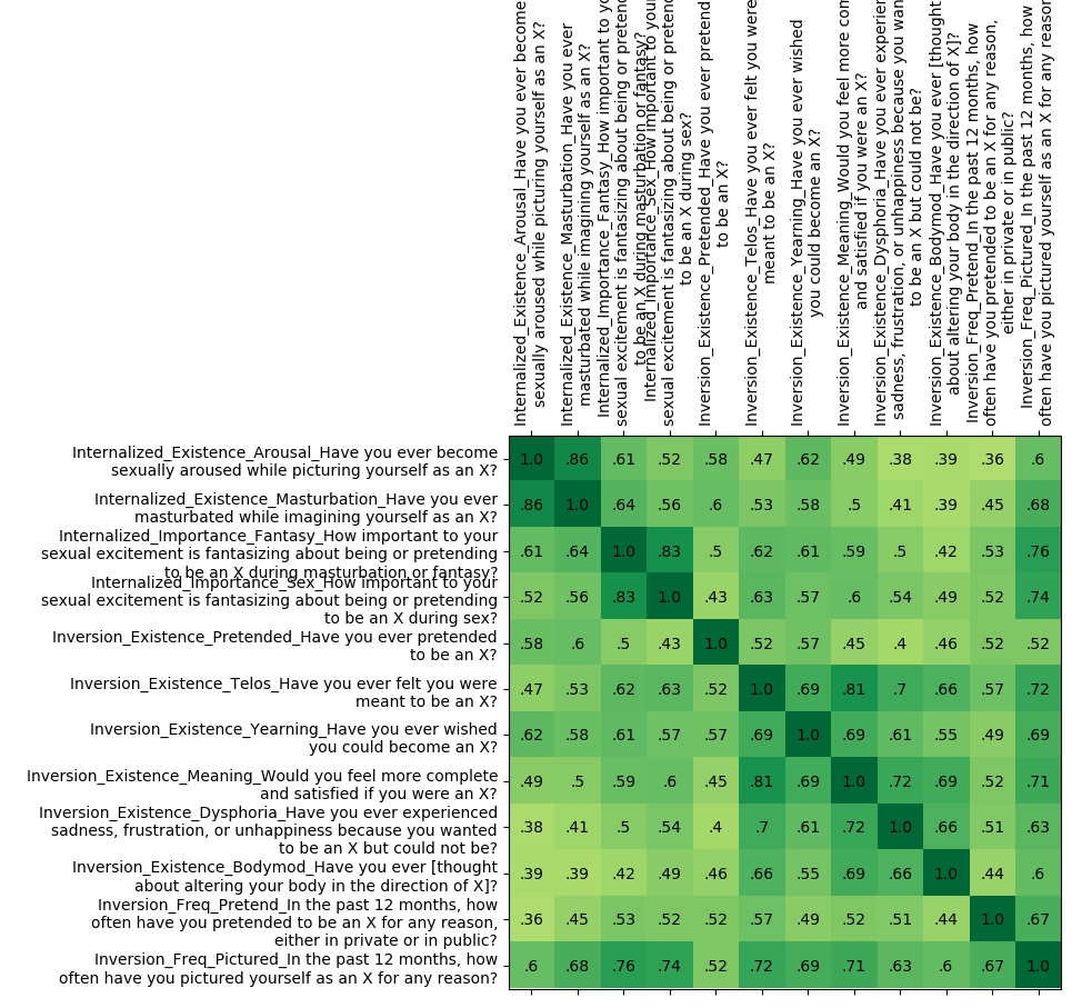
Let’s take a look at the correlations for the apotemnophilia items, as an example:

These items form two groups, which internally have much higher pairwise correlation than there is between the groups. That is, “Have you ever become sexually aroused while picturing yourself as an amputee?” and “Have you ever masturbated while imagining yourself as an amputee?” have a correlation of 0.86, and “How important to your sexual excitement is fantasizing about being or pretending to be an amputee during MASTURBATION or FANTASY?” and “How important to your sexual excitement is fantasizing about being or pretending to be an amputee during SEX?” have a correlation of 0.83, while the remained of the correlations are all below 0.65.

This goes back to the “We assume that the measurement error is independent of everything else” assumption that I brought up with Cronbach’s alpha. If the measurement error is independent of everything else, then the different items should only be correlated due to them reflecting the true level of apotemnophilia, and therefore the pattern of correlations should be very “uniform”, such that you wouldn’t see such big gaps. Furthermore it just intuitively makes sense that there would be correlated measurement error here, because the items are pairwise much more similar than they are across the pairs.

One way to eliminate these kinds of correlated measurement error is to first compose together the items that have correlated measurement error. This is called parceling, and the the resulting subscales are called parcels. All of the correlated measurement error should get embedded within each parcel, so that the remaining correlations between the parcels are hopefully just due to them reflecting the true level of apotemnophilia. When computing the alpha, rather than taking the X_is to be the individual items, one then takes them to be the parcels.

Since we can clearly see from the correlations that there is correlated measurement error, I think this kind of parceling is very well-justified, and so I will also do the same for my calculations. For apotemnophilia, I get an alpha of 0.78, and for BIID, I get an alpha of 0.88, and the correlation between the scores is 0.78, which turns into 0.95 after correcting for attenuation. These are basically in line with the researcher’s results, as would be expected from a direct replication of their methods. The results for the other ETIIs are similar, with me getting exactly the same correlations of 1.00 and 1.01 as Bailey et al did.

Further weakening the assumptions of Cronbach’s alpha

One of the key assumptions we made in deriving Cronbach’s alpha was the following:

This not only requires each indicator to split up into true level and measurement error, but also requires each indicator to be equally strongly affected by the true level, which seems like an unreasonably strong assumption, considering the different indicators are different questions (or question parcels), which have no particular reason to have Exactly Quantitatively Identical relationships to the outcomes. We might instead want to relax the assumption to something like:

… where a_i is some constant representing the degree of relationship between X_i and X.

Another key assumption was “we assume that var(ε_i) = var(ε_j)”. This similarly seems arbitrary; it says that the extent to which non-X factors influence each question must be the same regardless of what the question is. So for instance, questions about sex are not allowed to depend on any factors that questions about masturbation don’t also depend on. We might want to loosen things up by just dropping this assumption.

But if we drop these assumptions, then Cronbach’s alpha is no longer valid. There are some similar statistics, such as McDonald’s omega, which work similar to alpha without having such assumptions, but they are more involved and require too much linear algebra for me to even attempt to explain them here.

A simpler approach – albeit one that uses even heavier mathematical machinery than alpha or omega – is structural equation modelling. The idea in SEM is that you specify the relationships you think could be relevant, and then you let the computer find a model that fits the results.

Given the parceling that the researchers used, it seems like one can understand their model as being the following:

The fact that the researchers adjust for attenuation means that they see the items as being noisy indirect indicators of the underlying variables of Internalized Sexual Attraction and Identity Inversion, which we mark by placing them as distinct shapes and having causal arrows indicating that the latent variables influence the question responses. The fact that they do parceling means that they see the items as having correlated measurement error, which we mark by having bidirectional arrows between variables with measurement error.

I wrote up a computer program to do SEM, and entered this causal graph into the program. Unlike in the Cronbach alpha case, my program didn’t have arbitrary restrictions on the different indicators requiring them to have equal relationships to the latent variables, so it can compute the correction for attenuation in a more nuanced way.

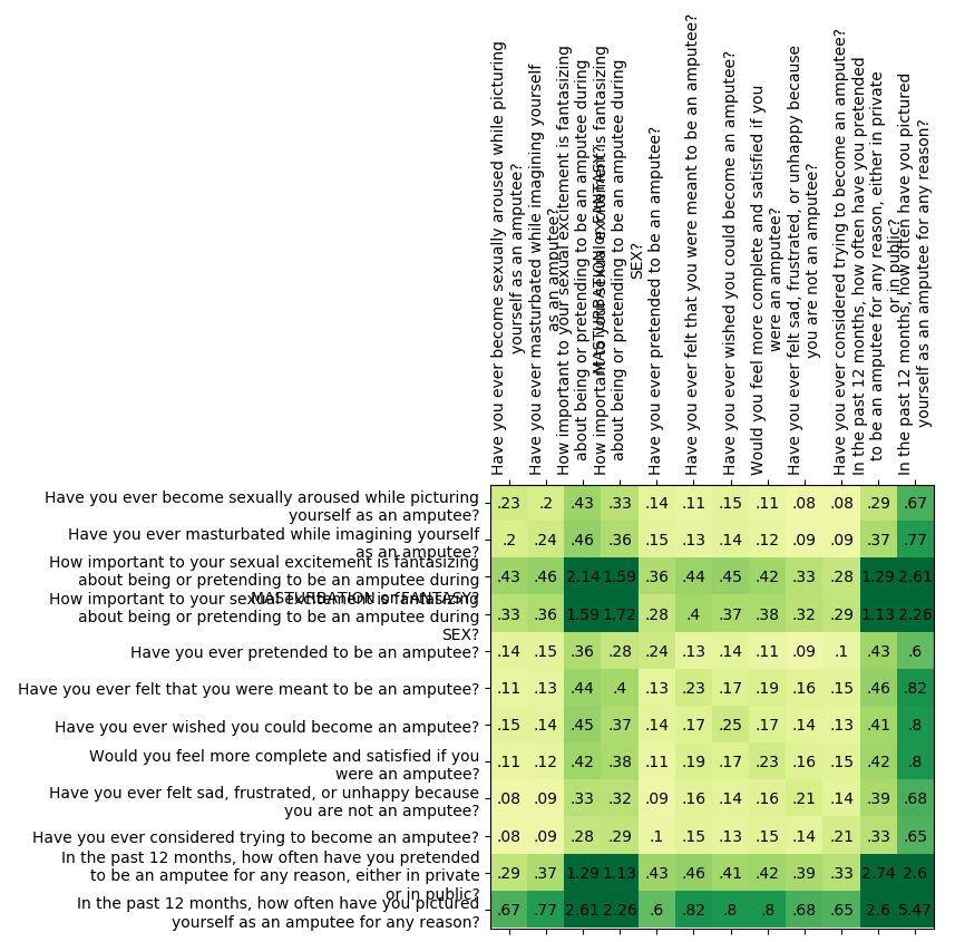
Roughly speaking, the way SEM works is that it adjusts the numbers in the model until the model’s predicted correlation matrix matches the correlation matrix observed in the data. So for example, here is the empirical correlation matrix for the apotemnophilia data:

Meanwhile, after fitting the model to make similar predictions, I end up with this predicted correlation matrix:

This SEM model replicates the results found with Cronbach’s alpha, that there is a correlation of 0.95 between apotemnophilia and BIID. If I run it for the other ETIIs, I similarly replicate the researchers’ results, and find correlations of 0.99 for autozoophilia/cross-species identity and 0.99 for autolipophilia/fat identity. The specific numbers for the SEM models can be seen here.

More correlated measurement error

Consider again the correlations for apotemnophilia/BIID:

The items “Have you ever pretended to be an amputee?” and “In the past 12 months, how often have you pretended to be an amputee for any reason, either in private or in public?” have a fairly high correlation, at 0.52. It is certainly a higher correlation than the 0.47 that the model predicts, presumably because they both ask about pretending to be an amputee. Thus to improve the model, I can let these have correlated measurement error.

Looking through the correlations, there were other items that seemed to have correlated measurement error, listed below.

The internalized existence items seemed to have correlated measurement error with:

• Have you ever pretended to be an X?
• If you could try being an X for one week, would you do it?
• Have you ever experienced sadness, frustration, or unhappiness because you wanted to be an X but could not be? (Negative correlation, mainly for lipophilia.)
• Have you ever wished you could become an X?

The “In the past 12 months, how often have you pretended to be a fat person for any reason, either in private or in public?” item seemed to have correlated measurement error with “Have you ever tried to gain weight in order to become a fat person?” for lipophilia, and as previously mentioned also with “Have you ever pretended to be an X?”.

Finally, there seemed to be a correlated measurement error between “How important to your sexual excitement is fantasizing about being or pretending to be an X during sex?” and “Have you ever wished you could become an X?”.

Adding all of these to the model, I get correlations of 0.95, 1.00, and 1.00 for acrotomophiles, zoophiles and lipophiles respectively. This suggests that Bailey et al’s results replicate well, though I should say that there is a lot of subjectivity in guessing which things do and do not have correlated measurement error, and I might not have been thorough enough to catch all of it. Furthermore, it appears that the study’s dataset contains a lot of extra identity and sexuality variables that could be used to pin down the model more precisely.

The specific numbers for the SEM models can be seen here.

Appendix

To make this more feasible for others to investigate, here are the covariance and correlation matrices for the items used in the study:

1. The chain only occurs under unknown conditions, e.g. most gynephilic males aren’t noticeably autogynephilic, so for ETII theory to be true there must be some unknown moderator of the gynephilia -> autogynephilia connection. ↩︎
2. I don’t really have a sufficiently quick way to convince you of this, so I would like for you to take it on faith. ↩︎